
A Post to Test Knitr to Jekyll
Remaining problems and observations
- Running servr::jekyll(daemon = TRUE) leads to the R console crashing. So we have to run servr::jekyll() and cannot use the console anymore.
- This behavior is also observed in the orinigal site from yihui.
- Preview in R Studio does not work
- it works fine in yihui’s site so the problem should be soved when analysing the differences between the two sites
- Figures (last part of this page) do not display nicely.
- Latex code like \(( x^2 + y^2 = 1 )\) now displays in HTML but will not render to PDF.
Test 6: succes! (sort of)
- put build.R in evflex
- put 2015-07-27-a-post-to-test-knitr-to-jekyll.Rmd in _source with output: html_document and remove all other content generated in earlier experiments with this file.
- run servr::jekyll() from the R console
- an empty viewer opens
- open the brower and surf to 127.0.0.1:4321
- The website opens and the post looks good (still no latex though)
- save new content
- it auto-refreshes in the browser
Test 5: as 4 but now in evflex again
- When we stop jekyll in the console and start it in powershell we see the post is there and has been given some layout but does not look as nice. E.g. source blocks are divided into separate lines.
Test 4: generate html with servr::jekyll() in Yihui’s repo
- as three but now from Yihui’s repro and after adding the laout: post tag to YaML.
- Much better! Liquid tags are also generated. However, no good Latex. Everything between \(this\) is simply ignored and the other stuff treated as text.
Test 3: generate html with servr::jekyll()
- put 2015-07-27-a-post-to-test-knitr-to-jekyll.Rmd in _source with output: html_document and remove all other content generated in earlier experiments with this file.
- run servr::jekyll() in the R Studio console
- a blank viewer is opened (showing html while there is only .md I presume)
- an .md file with the same name is created in _posts
- a directory with the same name is created in evflex/figure/source that contains png’s of the plots in the file.
- a directory with the same name is created in _site containing an index.html.
- we stop servr::jekyll() in the R console and start jekyll serve in powershell
- If we surf to 127.0.0.1:4000/filename the result is there but looks awful: yaml matter is missing and LaTex was ignored or the text is $shown as is$
- we stop servr::jekyll() in the R console and start jekyll serve in powershell
Test 2: generate md with servr::jekyll()
- put 2015-07-27-a-post-to-test-knitr-to-jekyll.Rmd in _source with output: md_document and remove all other content generated in earlier experiments with this file.
- run servr::jekyll() in the R Studio console
- a blank viewer is opened (showing html while there is only .md I presume)
- an .md file with the same name is created in _posts
- a directory with the same name is created in evflex/figure/source that contains a .png of the plots in the file.
- a directory with the same name is created in _site containing an index.html.
- we stop servr::jekyll() in the R console and start jekyll serve in powershell
- If we surf to 127.0.0.1:4000/filename the result is there but looks awful: yaml matter is missing and LaTex was ignored or the text is $shown as is$
- we stop servr::jekyll() in the R console and start jekyll serve in powershell
Test 1: plain Knit md_document
- put 2015-07-27-a-post-to-test-knitr-to-jekyll.Rmd in _source with output: md_document and remove all other content generated in earlier experiments with this file.
- Knit md into _source (push button)
- Run jekyll serve in directory evflex (branche gh-pages) in powershell
- Nothing happens: stop jekyll serve
- copy md_document and subfolder (figures) to _post.
- Run jekyll serve again
- Jekyll stops because it cannot handle cars-1.png (invalid byte sequence)
Original testcontent
This is an R Markdown document. Markdown is a simple formatting syntax for authoring HTML, PDF, and MS Word documents. For more details on using R Markdown see http://rmarkdown.rstudio.com.
When you click the Knit button a document will be generated that includes both content as well as the output of any embedded R code chunks within the document. You can embed an R code chunk like this:
summary(cars)## speed dist
## Min. : 4.0 Min. : 2.00
## 1st Qu.:12.0 1st Qu.: 26.00
## Median :15.0 Median : 36.00
## Mean :15.4 Mean : 42.98
## 3rd Qu.:19.0 3rd Qu.: 56.00
## Max. :25.0 Max. :120.00You can also embed plots, for example:
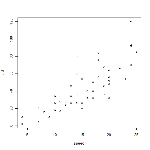
Note that the echo = FALSE parameter was added to the code chunk to prevent printing of the R code that generated the plot.
Some of my testcontent
Heading 1
Heading 2
Heading 3
Heading 4
- Bullet 1
- Bullet 2
- Lower level list
- Lower level list
- And back
LateX content
\[( x^2 + y^2 = 1 )\] \[\frac{d}{dx}\left( \int_{0}^{x} f(u)\,du\right)=f(x)\]Some more R code
Now we write some R code chunks in this post. For example,
install.packages(c('servr', 'knitr'), repos = 'http://cran.rstudio.com')options(digits = 3)
cat("hello world!")## hello world!set.seed(123)
(x = rnorm(40) + 10)## [1] 9.44 9.77 11.56 10.07 10.13 11.72 10.46 8.73 9.31 9.55 11.22
## [12] 10.36 10.40 10.11 9.44 11.79 10.50 8.03 10.70 9.53 8.93 9.78
## [23] 8.97 9.27 9.37 8.31 10.84 10.15 8.86 11.25 10.43 9.70 10.90
## [34] 10.88 10.82 10.69 10.55 9.94 9.69 9.62# generate a table
knitr::kable(head(mtcars))| mpg | cyl | disp | hp | drat | wt | qsec | vs | am | gear | carb | |
|---|---|---|---|---|---|---|---|---|---|---|---|
| Mazda RX4 | 21.0 | 6 | 160 | 110 | 3.90 | 2.62 | 16.5 | 0 | 1 | 4 | 4 |
| Mazda RX4 Wag | 21.0 | 6 | 160 | 110 | 3.90 | 2.88 | 17.0 | 0 | 1 | 4 | 4 |
| Datsun 710 | 22.8 | 4 | 108 | 93 | 3.85 | 2.32 | 18.6 | 1 | 1 | 4 | 1 |
| Hornet 4 Drive | 21.4 | 6 | 258 | 110 | 3.08 | 3.21 | 19.4 | 1 | 0 | 3 | 1 |
| Hornet Sportabout | 18.7 | 8 | 360 | 175 | 3.15 | 3.44 | 17.0 | 0 | 0 | 3 | 2 |
| Valiant | 18.1 | 6 | 225 | 105 | 2.76 | 3.46 | 20.2 | 1 | 0 | 3 | 1 |
(function() {
  if (TRUE) 1 + 1  # a boring comment
})()
## [1] 2names(formals(servr::jekyll)) # arguments of the jekyll() function## [1] "dir" "input" "output" "script" "serve" "command"
## [7] "..."Just to test inline R expressions1 in knitr, we know the first element in x (created in the code chunk above) is 9.44. You can certainly draw some graphs as well:
par(mar = c(4, 4, .1, .1))
plot(cars, pch = 19, col = 'red')  # a scatterplot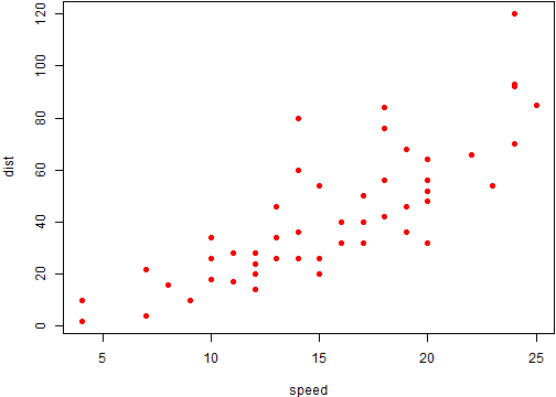
-
The syntax in R Markdown for inline expressions is
` r code`, wherecodeis the R expression that you want to evaluate, e.g.x[1]. ↩